Disclaimer: This example is taken from a reference titled ‘R In A Nutshell’ by Joseph A. Adler
In Machine Learning (ML), Regression is a supervised learning technique used to observe a correlation between variables (features/predictor) and to predict the continuous output (label/response) based on one or more variables. It is mainly used in prediction, forecasting, time-series modeling and determining the causal-effect relationship between variables.
One of the simplest technique of regression analysis is Linear Regression.
A linear regression assumes that there is a linear relationship between the response (label) variable and the predictor (features) variable
– R In A Nutshell, Joseph A. Adler
To study how linear regression works, let’s look at an example taken from the reference book. In this example, we are going to analyze a sample dataset collected on baseball teams scores.
First, load the lattice package.
library(lattice)Next, load the dataset.
load("team.batting.00to08.rda")I like to check the dimension of the dataset before I proceed, so that I have an idea of how big the dataset that I am going to work on.
> dim(team.batting.00to08)
[1] 270  13
Then, have a peek at the sample data in the dataset.
> head(team.batting.00to08)
  teamID yearID runs singles doubles triples homeruns walks stolenbases
1    ANA   2000  864     995     309      34      236   608          93
2    BAL   2000  794     992     310      22      184   558         126
3    BOS   2000  792     988     316      32      167   611          43
4    CHA   2000  978    1041     325      33      216   591         119
5    CLE   2000  950    1078     310      30      221   685         113
6    DET   2000  823    1028     307      41      177   562          83
  caughtstealing hitbypitch sacrificeflies atbats
1             52         47             43   5628
2             65         49             54   5549
3             30         42             48   5630
4             42         53             61   5646
5             34         51             52   5683
6             38         43             49   5644
Ok, now we are ready to begin our analysis. We are going to see how different features (metrics) such as singles, doubles, triples, homeruns, walks, stolenbases, caughtstealing, hitbypitch, sacrificeflies and atbats are related to the number of runs for each baseball team.
Let’s start with this;
runs~singles+doubles+triples+homeruns+walks+stolenbases
+caughtstealing+hitbypitch+sacrificeflies+atbats
A linear regression model suggested that;
y = I + C1x1 + C2x2 + C3x3 + ...

where I is the Interceptor and C is the Coefficient, while y is the response and x is the predictors.
Before we train the data, we are going to transform it into a data frame first.
attach(team.batting.00to08)

forplot <- make.groups(
    singles = data.frame(value=singles, teamID,yearID,runs),
    doubles = data.frame(value=doubles, teamID,yearID,runs),
    triples = data.frame(value=triples, teamID,yearID,runs),
    homeruns = data.frame(value=homeruns, teamID,yearID,runs),
    walks = data.frame(value=walks, teamID,yearID,runs),
    stolenbases = data.frame(value=stolenbases, teamID,yearID,runs),
    caughtstealing = data.frame(value=caughtstealing,teamID,yearID,runs),
    hitbypitch = data.frame(value=hitbypitch, teamID,yearID,runs),
    sacrificeflies = data.frame(value=sacrificeflies,teamID,yearID,runs)
    )

detach(team.batting.00to08)
Then, plot it so that we can observe the distributions of the data.
xyplot(runs~value|which, data=forplot,
       scales=list(relation="free"), pch=19, cex=.2,
       strip=strip.custom(strip.levels=TRUE,
                          horizontal=TRUE,
                          par.strip.text=list(cex=.8)))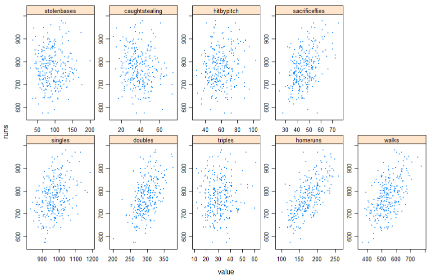
Based on the plot, we can see that as predicted, teams that hit a lot of homeruns definitely score more runs. Eventually, teams that walks also able to score more runs as well. Interesting.
Next, training the data so that we can check out our hypotheses about the relationship between the features (singles, doubles, homeruns, etc.) and the number of runs for each team. For training, we are going to use the lm function.
runs.mdl <- lm(formula=runs~singles+doubles+triples+homeruns+walks+hitbypitch+sacrificeflies+stolenbases+caughtstealing, data=team.batting.00to08)View the model returned.
> runs.mdl

Call:
lm(formula = runs ~ singles + doubles + triples + homeruns +
    walks + hitbypitch + sacrificeflies + stolenbases + caughtstealing,
    data = team.batting.00to08)

Coefficients:
   (Intercept)         singles         doubles         triples        homeruns
    -507.16020         0.56705         0.69110         1.15836         1.47439
         walks      hitbypitch  sacrificeflies     stolenbases  caughtstealing
       0.30118         0.37750         0.87218         0.04369        -0.01533
Use the summary function to get the summary of the linear model object.
> summary(runs.mdl)

Call:
lm(formula = runs ~ singles + doubles + triples + homeruns +
    walks + hitbypitch + sacrificeflies + stolenbases + caughtstealing,
    data = team.batting.00to08)

Residuals:
    Min      1Q  Median      3Q     Max
-71.902 -11.828  -0.419  14.658  61.874

Coefficients:
                 Estimate Std. Error t value Pr(>|t|)
(Intercept)    -507.16020   32.34834 -15.678  < 2e-16 ***
singles           0.56705    0.02601  21.801  < 2e-16 ***
doubles           0.69110    0.05922  11.670  < 2e-16 ***
triples           1.15836    0.17309   6.692 1.34e-10 ***
homeruns          1.47439    0.05081  29.015  < 2e-16 ***
walks             0.30118    0.02309  13.041  < 2e-16 ***
hitbypitch        0.37750    0.11006   3.430 0.000702 ***
sacrificeflies    0.87218    0.19179   4.548 8.33e-06 ***
stolenbases       0.04369    0.05951   0.734 0.463487
caughtstealing   -0.01533    0.15550  -0.099 0.921530
---
Signif. codes:  0 ‘***’ 0.001 ‘**’ 0.01 ‘*’ 0.05 ‘.’ 0.1 ‘ ’ 1

Residual standard error: 23.21 on 260 degrees of freedom
Multiple R-squared:  0.9144,	Adjusted R-squared:  0.9114
F-statistic: 308.6 on 9 and 260 DF,  p-value: < 2.2e-16
Here’s the ANOVA statistics for the model.
> anova(runs.mdl)
Analysis of Variance Table

Response: runs
                Df Sum Sq Mean Sq   F value    Pr(>F)
singles          1 215755  215755  400.4655 < 2.2e-16 ***
doubles          1 356588  356588  661.8680 < 2.2e-16 ***
triples          1    237     237    0.4403  0.507565
homeruns         1 790051  790051 1466.4256 < 2.2e-16 ***
walks            1 114377  114377  212.2971 < 2.2e-16 ***
hitbypitch       1   7396    7396   13.7286  0.000258 ***
sacrificeflies   1  11726   11726   21.7643 4.938e-06 ***
stolenbases      1    357     357    0.6632  0.416165
caughtstealing   1      5       5    0.0097  0.921530
Residuals      260 140078     539
---
Signif. codes:  0 ‘***’ 0.001 ‘**’ 0.01 ‘*’ 0.05 ‘.’ 0.1 ‘ ’ 1
Based on the statistics, it appears that triples, stolenbases and caughtstealing are not significant to the number of runs scored by each team.
Click here to download the dataset.